Parametric Variable Thickness Wall Tutorial

This tutorial will show how to create a parametric variable thickness wall using two input curves and a point attractor using Rhino 5 and Grasshopper 0.9 and PanelingTools for Grasshopper.
This is how the result looks:

INPUT
The input includes:
- Two curves and the attraction point.

- Variable offset distance (relative to the attractor point) that ranges between 2 and 5.

STEPS
In order to solve the problem, we will need the following steps:
1- Create tween curves between the two input curves
2- Divide the curves to create a first grid
3- Offset the grid in the normal direction and variable distance.
4- Populate a unit pattern between the two grids

SOLUTION
1- We will use the "TweenCrv" component to define the list of curves.

• Inputs "A" and "B" represent the two input curves.
• Input "F" represents the distance factor between 0.0 ( which create a tween curves that overlaps curve A) and 1.0 (overlaps curve B).
• We will need to generate a list of factors between 0.0 and 1.0 and we will use the "Range" component for it. Keep the default domain "D" (0-1):

2- For the grid, we can use GH standard divide curve, or use one the curve divide components in the PanelingTools for Grasshopper add-on as in the following.

3- We will need a surface to help us evaluate the normal offset directions of the grid points. We will use a PanelingTools component (ptGridSurface) to create a surface that goes through the grid of points. Make sure to set input "T" to "True".

    Now we can calculate the normal directions of each one of the grid points as follows:

    Now that we have the normals, we need to decide the offset distance for each point using the point attractor. For that, we need to create the grid that represents the degree of attraction.  We will do that using the PanelingTools "ptPointAtt" component. Note that the result "W" is always between 0-1.

We need to map the domain of values from 0-1 to 2-5.  We will use and "Expression" component for that. Notice how the domain of values changed to 2-5.

The final step is to change the amplitude of the normal vectors based on the attraction and use to offset grid points.  Make sure that the input to the GH "Move" component is compatible. In our example, we have two tree structure inputs.  The first is for the geometry "G" and the second is for the vectors "T".  We need to "Simplify" the "G" input to match the "T" input. We do that by "right-mouse click" the "G" input and select the "Simplify" option.

4- The final step involves creating the unit pattern and morph it between the two bounding grids. We will use the PanelingTools "ptMPanel3D" component.  It takes two bounding grids "Gd1" and "Gd2", the unit shift in the "i" and "j" directions, and a list of strings representing unit connections:

    The "ptMPanel3D" component takes a list of strings representing unit-pattern connections.  For example, the above two strings represent a partition cross module.  Here is an illustration of how it works:

Digital Sketching with PanelingTools

The following is a recording of part of an invited lecture at Savannah College of Art and Design (Feb 2012). It covers the use of PanelingTools as a tool to sketch paneling patterns.

Parametric Curves - Basic Concepts

This article explains few basic concepts related to parametric curves using Rhino 5 and Grasshopper 0.9.

CURVE PARAMETER
Parametric curves are defined using a parameter. Think of a parametric curve as a path traveled between two points.  If traveling takes T amount of time, then the parameter "t" represents any point in time within T, where the traveler will be at some point within the path.

For example, the parametric line equation is defined as:
P = P0 + t*v
where
P: is any point on the line
P0: is a given point on the line
t: is a parameter on the line, and
v: is a vector and represents the direction of the line.

Now suppose we have a straight path (linear curve) between the two points A and B, and v was a vector from A to B (v=B-A). We can use the parametric line equation to find all points "M" between A and B using the parametric line equation above:
M = A + t*(B-A)
where
t: is any value between 0 and 1

The range of "t" values, which are 0 to 1 in this case, is referred to as the curve "domain" or "interval".  If "t" was a value outside the domain (less that 0 or more than 1 in this case), then the resulting point M will be outside the linear curve AB.

CURVE DOMAIN:
A curve domain is defined as the range of parameters that evaluate into a point within that curve. The domain is usually described as two real numbers (min to max) or (min,max).  The domain limits can be any two values that may or may not be related to the curve actual length. However, it is very common that the domain be set to (0 to 1).

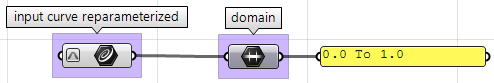
Changing a curve domain is referred to as "reparameterize" the curve. In Grasshopper, you can set the curve domain to (0 to 1) using the "Reparameterize" option on any curve input. Also there is a Rhino command "Reparamterize" that allows you to set any min and max domain values. The following example in GH reparameterize the above curve domain to be (0-1):

An increasing domain means that the minimum value of the domain points to the start of the curve. Domains are typically increasing, but not always.

EVALUATE A CURVE
Evaluating a curve at a parameter that is within the curve domain results in a point that is "on" the curve. The following example curve has a domain (0 to 1). It shows how to evaluate the curve at mid-domain parameter (t = 0.5). Notice that parameter value that is in the middle of the domain might not evaluate into the middle point along the curve.

That brings us to the concept of parameter density of a parametric curve.  Using the traveling metaphor used above, you can think of uniform parameter density of a curve as traveling a path with constant speed.  It is though possible (and more likely) that the speed decreases or increases along the path.  For example, if it takes 30 minutes to travel a road, it is unlikely that you will be exactly half way through at minute 15. However, there are times when you need to evaluate points on a curve that are at a defined percentage of the curve length.  For example, you might need the mid point of a curve. In order to achieve that, you need to find the parameter "t" at mid point and then evaluate the curve at that parameter. This parameter is called "normalized parameter". The following example evaluates a normalized mid domain parameter (t=0.5) for a curve that has domain (0 to 1).

TANGENT VECTOR TO A CURVE
A tangent to a smooth curve at any parameter (or point) is the vector that touches the curve at that point, but does not cross over.  The slope of the tangent vector equals the slope of the curve at the same point. The following example evaluate the tangent at the two points defined in the above two examples.

Vector Display Tutorial

The first exercise was to create a vector that points to the positive "Y" direction and has a length equal to "5" units. 

Knowing a vector is a direction and magnitude we need to start in a point defined in space, for this example we will use point (0,0,0) 

Now to get point (0,0,0) We need to define that point in grasshopper, so we use either a panel [command: panel] or a number slider [command: type in any number] 

We will define these sliders as 0 to get the coordinate (0,0,0), label X, Y, and Z to keep the definition readable for when the definition gets larger and you need to reference back to this point for easier access. 

Next we create a vector with three input points X,Y,Z 

To do this we need to create our own vector, and this is simple because we already have the anchor point to the vector. Now we just need to actually define the vector based off those coordinates. to do this we need the vectorXYZ component This can be found under; top menu bar, Vector --> Vector --> VectorXYZ  or [Command: Vector XYZ] 

Input:

XYZ

Output:

V: Vector

L: Length

We now have a vector  point but no magnitude and at this point should not be visible in the rhino screen, this is normal. 

To display this vector point we need a vector display, to do this we need the vector display component 

to get this component go to;  top menu bar, Vector --> Vector --> Vector Display or [Command: Vector Display] 

Input:

A: Anchor

V: Vector

To view your anchor point plug in your Vec: V to VDis: A

Your point should now be visible

Next we have to create a magnitude and direction for this vector anchor point

To do this copy and paste your number sliders and Vector XYZ components, then take the output of the Vec: V and and plug this into the input VDis:V 

You should now have a Vector with a magnitude in the X,Y,Z coordinates, to change this vector, you can now move any of the sliders to now have a changing vector which is an integral part in parametric design within grasshopper

Below are two examples of different vector configurations, to get multiple vectors copy and paste the whole single definition.

Tangent Spheres Tutorial

This tutorial will show how to create two tangent spheres between two input points using Rhino 5 and Grasshopper 0.9.
This is how the result looks:

INPUT
The input here is two points in the 3D coordinate system.  Let us call them points A and B.

PARAMETERS
This is a diagram of the parameters that we will need in order to solve the problem:

1- A tangent point D between the two spheres, at some "t" parameter (0-1) between points A and B.
2- The center of the first sphere, or the mid point C1 between A and D.
3- The center of the second sphere, or the mid point C2 between D and B.
4- the radius of the first sphere (r1), or the distance between A and C1.
5- The radius of the second sphere (r2), or the distance between D and C2.

SOLUTION
We need to define or generate all the parameters identified in the above.
1- We will use the "Expression" component to define point D between A and B at some parameter t. The expression we will use is based on the vector equation of a line: D = A + t*(B-A).

• B-A: is the vector that goes from B to A using vector subtraction operation.
• t*(B-A): where "t" value is between 0 and 1 to get us a location on the vector.
• A+t*(B-A): gets a point on the vector between A and B.

2- We will use the "Expression" component to also define the mid points C1 and C2.
.

3- The first sphere radius (r1) and the second sphere (r2) can be calculated using the "Distance" component.

4- The final step involves creating the sphere from a base plane and radius. We need to make sure the origins are hooked to C1 and C2 and the radius from r1 and r2.

Exploded Box Tutorial

The following tutorial will show how to explode a polysurface using Rhino 5 and Grasshopper 0.9.
This is how the final exploded box looks like:

INPUT
First we need to identify the input, which is a box in this case.
We will use the "Box" parameter in GH:

PARAMETERS
Next, we need to think of all the parameters we need to know in order to solve this tutorial.
1- The center of explosion,
2- The box faces we are exploding,
3- The direction in which each face is moving.

Once we have identified the parameters, it is a matter of putting it together in a solution.

SOLUTION
Let us put together the solution. Basically piece together the logical steps to reach an answer:
1- The center of the box can be found using the "Box Properties" component in GH:

2- Box faces can be extracted from "Deconstruct Brep" component:

3- The direction in which we move the faces is the tricky part.  We need to first find the center of each face, then define the direction from the center of the box towards the center of each face as in the follows:

4- Once we have all the parameters scripted, we can use the "Move" component to move the faces in the appropriate direction.  Just make sure to set the vectors to the desired amplitude, and you will be good to go.
Here is how the final solution looks:

Welcome to NSAD AGG

Welcome to the architectural geometry and computational design group at Newschool of Architecture + Design in San Diego, California. The blog is meant to share knowledge and showcase our students' designs and experiments with the digital medium of design. In the process, we hope to introduce the foundation knowledge in the field and also explore available technologies and processes used in digital design and fabrication in architectural education and the practice of architecture today.